Central Limit Theorem

The Central Limit Theorem states that the sample means will be approximately normally distributed for a large sample size regardless of the distribution from which the sample is taken.

Assume you are sampling from a population with mean $\mu$ and standard deviation of $\sigma$ and let $\overline{X}$ be representing sample mean of $n$ of independently drawn observations, then

The mean of the sample distribution of the sampling distribution of the sample means is equal to the population mean.

$\mu \overline{x} = \mu$

The standard deviation of the sampling distribution of $\overline{X}$ is equal to:

$\sigma \overline{x} = \frac {\sigma}{\sqrt{n}}$

Now, If the population is normally distributed, then $\overline{X}$ is also normally distributed.

What if the population is not normally distributed?

The central limit theorem addresses this question.

The distribution of the sample mean tends toward normal distribution as the sample size increases, regardless of the distribution from which we are sampling.

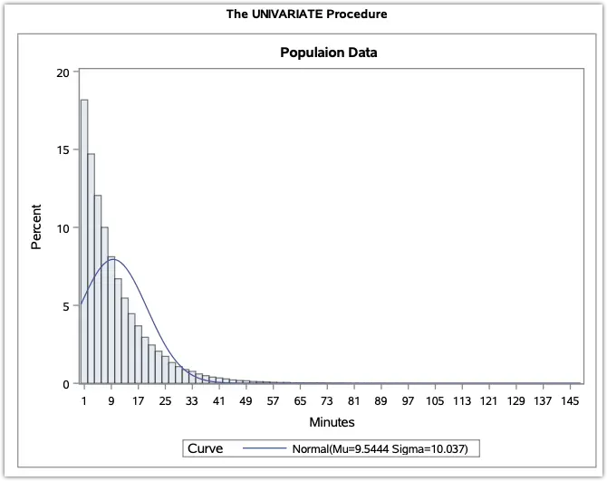
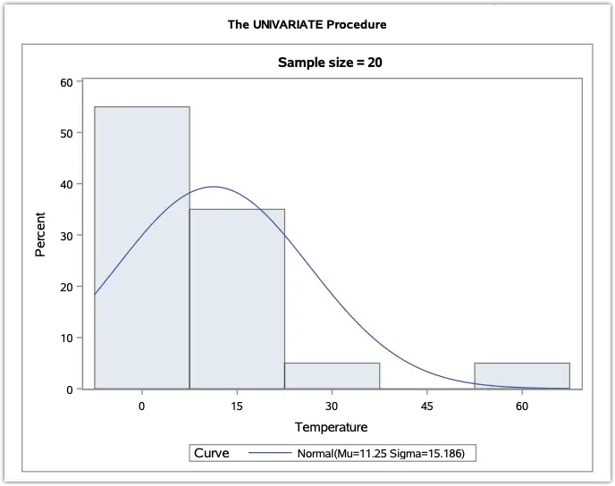
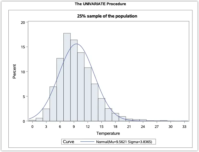
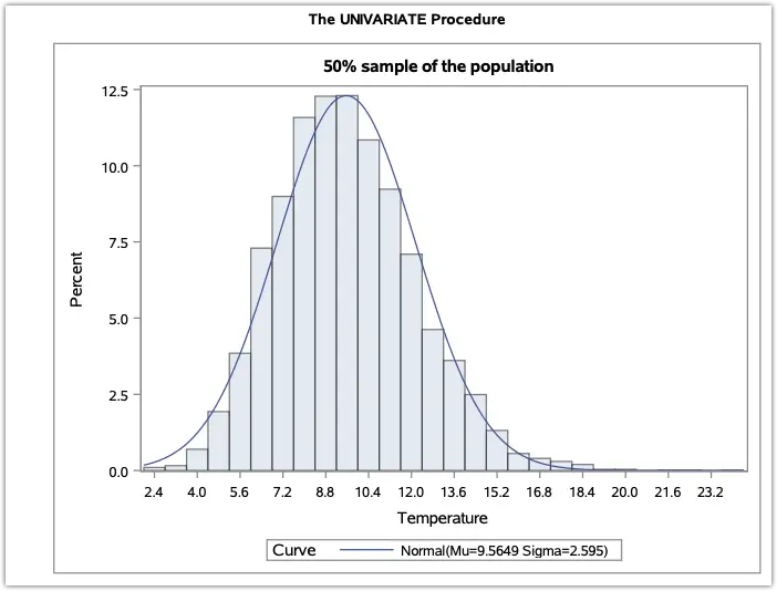
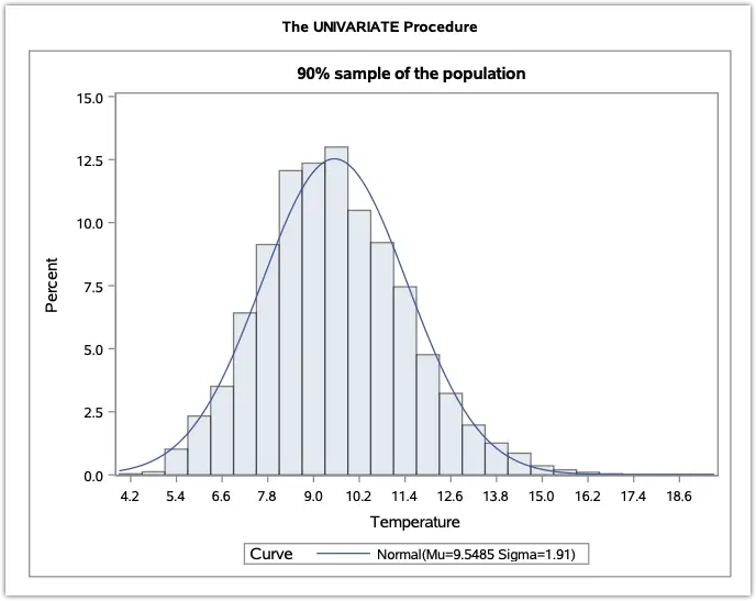
You may refer to an example of the Central Limit Theorem in the link below.

http://sasnrd.com/sas-central-limit-theorem/

Properties of Central Limit Theorem

The variable $\frac{X- \mu}{\sigma/\sqrt(n)}$ will be a standard normal distribution where mean = 0 and standard error = 1.
The sampling distribution of a large sample where $(n > 30)$ will follow the normal distribution with the mean same as the population mean and standard deviation $\sigma \sqrt{n}$
The mean of sample means will be equal to the mean of the population which means if you take the average of all sample means, it will be equal to the average of the population. Note that this depends on the sample size.
If the Population is normally distributed, then the mean of the sample will be normal irrespective of the sample size.

Central Limit Theorem for proportions

Example:

It is believed that college students spend on average 65.5 minutes daily texting using their cell phone and the corresponding standard deviation is 145 minutes. Data from 100 students were collected to calculate the amount of time spent on texting.

Calculate the probability that the average time spent by this sample of students will exceed 90 minutes.

Solution:

Using the Central limit theorem, the mean of the sampling distribution is 65.5, and the formula calculates the corresponding standard deviation.

$\sigma \overline{x} = \frac {\sigma}{\sqrt{n}}$

Standard Deviation (For sample) = $145/\sqrt{100} = 14.5$

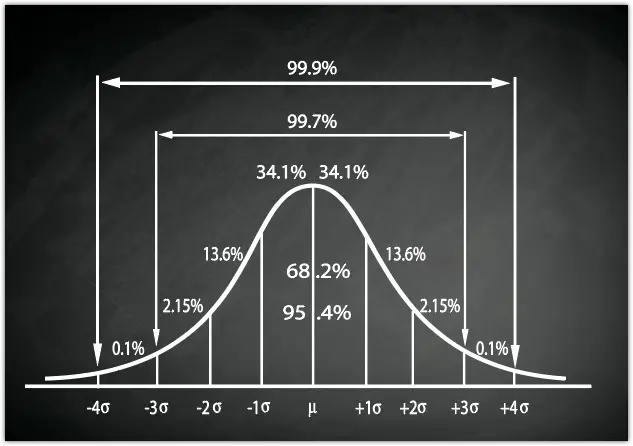
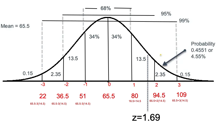
We can assume that the Z score will lie somewhere between a standard deviation of 1 and 2, that is (65.5 + 14.5), which is 80 and (65.5+2*(14.5)), which is 90. (See the graph below)

Now, I will calculate the Z score.

The Z score is calculated using.

$z = \frac {x - \mu}{\sigma}$

$z = \frac {90-65.5}{14.5} = 1.69$

From the empirical rule of 99.7%-95%-68%, we can assume the probability is somewhere between 13.5% and 3.50 (0.15+2.35). (See the graph below)

We can find the Probability or area under the curve using a Z table with the probability calculated for Z values ranging from -3.49 to +3.49.

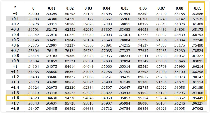
You must find the value P-value by looking at the left column for 1.6 and 0.09 from the Z table for 1.6 and 0.09 from the top column. We get P as 0.954. Since I have found the area for +ve Z, we have to subtract this value by 1. So, the probability will be (1-0.95449)= 0.04551.

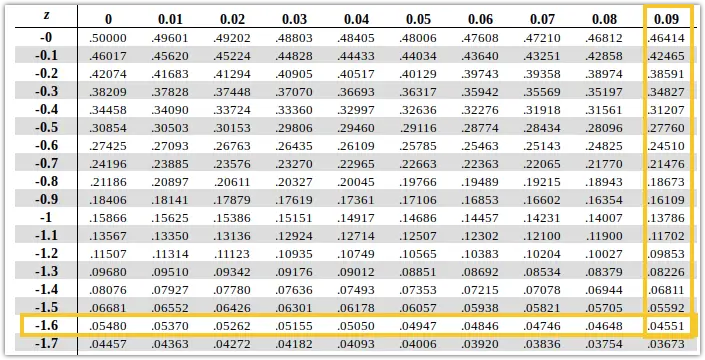
You can also look at the -1.69 Z score and get the P-value directly, the same as above.

So, I could say that the probability of exceeding 90 minutes is 4.55%.

Calculating Probability in SAS

To calculate the probability and the z score, you can use the probnorm function in SAS as below.

DATA NORMAL;
 MU=65.5;
 SIGMA=14.5;
 Y=90;
 Z=(Y-MU)/SIGMA;
 PROBABILITY=1- PROBNORM(Z);
RUN;

Central Limit Theorem

Properties of Central Limit Theorem

Central Limit Theorem for proportions

Calculating Probability in SAS

Subhro

Leave a ReplyCancel reply