Using PROC MEANS for detailed analysis of data.

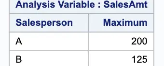
PROC MEANS, PROC SUMMARY and PROC FREQ in SAS are used to evaluate quantitative data and to create a summary report for analysis. Using the PROC MEANS procedure, you can compute statistics like finding the mean, standard deviation, minimum and maximum values and a lot more statistical calculations.

Applications of PROC MEANS

• Describing quantitative data for analysis.
• Describing the means of numeric variables by group
• Identifying outliers and extreme values.

SYNTAX

PROC MEANS DATA=dataset-name ;
  BY  variables;
  CLASS variable(s) / ;
  VAR variables;  
  OUTPUT OUT=SAS-data-set ;
RUN;

The explanation of statements of PROC MEANS is as follows :

PROC MEANS DATA=dataset-name;:

• PROC MEANS: Initiates the PROC MEANS procedure.
• DATA=dataset-name: Specifies the name of the dataset to be analyzed.

BY variables;:

• BY: Indicates that the dataset is sorted by the specified variables, and separate analyses should be produced for each unique combination of the BY variables.
• variables: Lists the variables by which the dataset is sorted.

CLASS variable(s) / options;:

• CLASS: Indicates the start of the list of classification variables.
• variable(s): Specifies one or more classification variables. The procedure will produce separate analyses for each unique combination of the CLASS variable levels.
• / options: Specifies options for the CLASS statement. For example, MISSING includes missing values as a valid level.

VAR variables;:

• VAR: Indicates the start of the list of variables to be analyzed.
• variables: Lists the variables to be analyzed.

OUTPUT OUT=SAS-data-set;:

• OUTPUT: Indicates that summary statistics should be written to an output dataset.
• OUT=SAS-data-set: Specifies the name of the output dataset where the summary statistics will be saved.

In this syntax, PROC MEANS analyzes the specified VAR variables from the given dataset, producing summary statistics for each unique combination of the BY variables and each unique combination of the CLASS variable levels. The resulting summary statistics are then saved to the specified output dataset.

Common Statistical Options of PROC MEANS

Here’s a table listing the statistical options used in PROC MEANS:

Option	Description
N	Number of non-missing values
NMISS	Number of missing values
SUM	Sum of values
MEAN	Arithmetic mean
STD	Standard deviation
STDERR	Standard error of the mean
VAR	Variance
CV	Coefficient of variation
MIN	Minimum value
MAX	Maximum value
RANGE	An unbiased estimate of sum of squares
CLM	Confidence limits for the mean
USS	An unbiased estimate of the sum of squares
CSS	Corrected sum of squares
T	t Value
PROBT	Probability of the t value
SKEWNESS	Skewness
KURTOSIS	Kurtosis
LCLM	Lower confidence limit for the mean
UCLM	Upper confidence limit for the mean
MODE	Mode
QRT	Quartiles
MEDIAN	Median (50th percentile)
PRT	Percentiles

These options can be specified in the PROC MEANS statement to request the desired statistics. For instance, to obtain the mean, standard deviation, and range.

Statistical keywords are used to calculate mean, median and standard deviation measures. You can find the list of Statistical keywords on the SAS documentation website.

In addition to the primary statistical options listed above, PROC MEANS offers several other features and options to enhance its functionality:

Option	Description
AUTONAME	Generates variable names for output dataset
ALPHA	Specifies the level of confidence
NWAY	Produces only the grand total for CLASS variables
TYPES	Produces output for specified combinations of CLASS variables
WAYS	Produces output for up to n-way combinations of CLASS variables
ORDER	Specifies the order for levels of CLASS variables
ID	Identifies observations in printed output
OUTPUT	Outputs summary statistics to a dataset
PRINT	Controls the printing of results
SUMSIZE	Specifies the maximum amount of memory for summarizing data

Difference between PROC MEANS and PROC SUMMARY

The difference between PROC MEANS and PROC SUMMARY is that: By default, MEANS always creates a table to be printed. If you do not want a printed table, you must explicitly turn it off (NOPRINT option). On the other hand, the SUMMARY procedure never creates a printed table unless it is specifically requested (PRINT option).

The CLASS statement.

The CLASS statement in PROC MEANS allows for the categorization of data. It enables the calculation of statistics for individual groups within a dataset.

The order of variables in the CLASS statement determines the order of classification of variables.

Options can be applied in the CLASS statement by preceding the option with a slash.

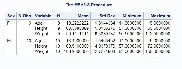
PROC MEANS DATA = sashelp.class;
CLASS sex;
RUN;

The VAR Statement

The VAR statement specifies the variables for which PROC MEANS calculates statistics.

PROC MEANS DATA = sashelp.demographics;
CLASS region;
VAR pop;
RUN;

The OUTPUT Statement

The OUTPUT statement creates a new dataset containing the calculated statistics.

PROC MEANS DATA = sashelp.demographics;
CLASS region;
VAR pop;
OUTPUT OUT = stats mean=;
RUN;

The MISSING Option

The MISSING option in PROC MEANS is used to treat missing values as valid category levels for classification variables specified in the CLASS statement.

By default, PROC MEANS excludes observations with missing values for the classification variables. However, when you use the MISSING option, PROC MEANS includes these observations and treats the missing values as a valid category.

Let’s go through an example to understand the MISSING option:

Suppose we have a dataset of students’ scores, but, some students didn’t specify their subject:

data scores;
input StudentID $ Subject $ Score;
datalines;
001 Math 85
002 . 90
003 Math .
001 Science 88
002 Science 92
003 . 86
;

Notice that Student 002 didn’t specify the subject for one of their scores, and Student 003 has a missing subject for their score of 86.

Without the MISSING option:

proc means data=scores mean;
   class Subject;
   var Score;
   output out=WithoutMissing mean=;
run;

proc print data=WithoutMissing; run;

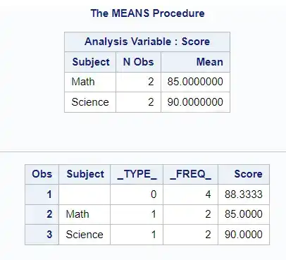
This will compute the mean score for each subject, but it will exclude the observations with missing scores.

Using the MISSING option:

proc means data=scores mean missing;
   class Subject;
   var Score;
   output out=WithMissing mean=;
run;

proc print data=WithMissing; run;

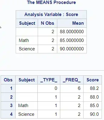
With the MISSING option, PROC MEANS will include the observations with missing scores when computing the mean. The output will show the mean score for each subject, including the observations with missing scores.

In summary, the MISSING option in PROC MEANS allows you to include observations with missing values for classification variables in the analysis, treating the missing values as a valid category level.

<span class="token step keyword">data</span> <span class="token keyword">class;</span> <span class="token keyword">set</span> sashelp<span class="token punctuation">.</span>class<span class="token punctuation">;</span> <span class="token keyword">if</span> age <span class="token operator"><</span> <span class="token number">14</span> <span class="token keyword">then</span>  age<span class="token operator">=.;</span>run<span class="token punctuation">;</span>

Note: The MISSING option in PROC MEANS is primarily impactful when used with the CLASS statement. It treats missing values in the classification variables as a valid category. However, for the analysis variables (like Score in our example), PROC MEANS always excludes the missing values when calculating statistics, regardless of whether the MISSING option is used.

Options in the CLASS Statement

When working with the CLASS statement in Proc, you have the flexibility to specify multiple variables for analysis. This enables you to explore and analyze the relationship between different categorical variables and the outcome of interest in your data.

You can use the below option with the class statement. To use the options in a CLASS statement, you must use the ORDER of the classification variables.

Changing the Displayed Order of the Classification Variable

These options allow you to reverse the order of the display values accordingly.

proc means data=class;
 class age /order=freq ascending;
run;

ORDER

With this option, you can control the classification variable levels. There are options by which you can determine the order. Below are the options which you can use with the ORDER statement.

• DATA – order is based on the order of incoming data
• FORMATTED – Values are formatted first and then ordered.
• FREQ – the order is based on the frequency of class level.
• INTERVAL – It is the same as UNFORMATTED or GROUPINTERVAL

<span class="token step keyword">proc means</span> <span class="token proc-args"><span class="token arg keyword">data=class2;</span></span> <span class="token keyword">class</span> age bmi<span class="token operator">/</span>order<span class="token operator">=</span>freq<span class="token punctuation">;</span> <span class="token keyword">var</span> height weight<span class="token punctuation">;</span>run<span class="token punctuation">;</span>

GROUPINTERVAL and EXCLUSIVE

With these options, you can determine the formats associated with CLASS variables when forming groups.

When a classification variable is associated with a format, that format is used in forming the groups.

In the following example, the format weight class is used to classify students (Normal, Overweight, Underweight) based on their BMI.

proc format;
 value weightClass low - 18.5='Underweight' 18.6-24.9='Normal' 
  25 - 29.9='Overweight' 30 - high='Obese';
run;
data class2;
 set sashelp.class;
 bmi=weight*703/(height**2);
 format bmi weightclass.;
run;
proc means data=class2 noprint;
 class bmi/groupinternal;
 var height weight;
 output out=class_summary
 mean = MeanHT MeanWT;
run;

The resulting output shows that the MEANS procedure has used the format to collapse the individual BMI levels into the three formatted classification variable levels.

MLF

Multilevel formats allow you to have overlapping formatted levels.

In addition to the ORDER option, other useful options can enhance your analysis when using the CLASS statement. For instance, the REF option allows you to specify a reference level for your classification variables, which can serve as a baseline for comparison against the other levels. This is particularly helpful when you want to investigate how different levels of a categorical variable compare to a specific reference level.

Furthermore, the EFFECT option in the CLASS statement allows you to generate parameter estimates for the individual levels of a categorical variable, providing valuable insights into the impact of each level on the outcome variable. This can be particularly useful in predictive modelling or understanding the influence of different categories on a particular metric.

OUTPUT options in Proc Means

The OUTPUT statement with the OUT= option stores the summary statistics in a SAS dataset. There are other options which you can use on the OUTPUT statements.

• AUTONAME – This allows the MEANS and SUMMARY to determine names for the generated variables.
• AUTOLABEL – Allows MEANS and SUMMARY to apply a label for each generated variable.
• LEVELS – Adds the LEVELS column to the summary data set.
• WAYS – Add the WAYS column to the summary dataset.

The difference between BY and CLASS Statements

The input dataset must be sorted by the BY variables whereas in CLASS variables it is not required to sort the data. The BY statement provides summaries for the groups created by the combination of all BY variables. whereas the CLASS statement will provide summarized values for each class variable separately and also for each possible combination of class variables unless you use the NWAY option.

You can also use the CLASS and BY statements together to analyse the data by the levels of class variables within BY groups.

Calculating Basic Statistics

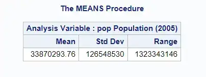
PROC MEANS can calculate a variety of statistics. For example, to calculate the mean, standard deviation, and range of the population in a dataset, the following code could be used:

PROC MEANS DATA = sashelp.demographics MEAN STD RANGE;
VAR pop;
RUN;

Grouping Data with CLASS Statement

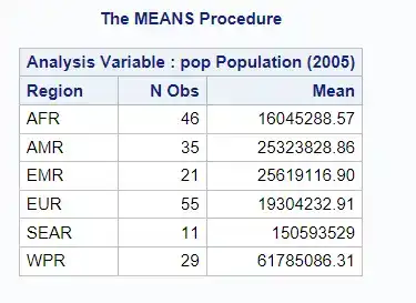
The CLASS statement allows for the calculation of statistics for individual groups. For example, to calculate the mean population in each region, the following code could be used:

PROC MEANS DATA = sashelp.demographics MEAN;
CLASS region;
VAR pop;
RUN;

Adding Multiple Classification Variables

Changing the Displayed Order of the Classification Variable

Creating Output Data with OUTPUT Statement

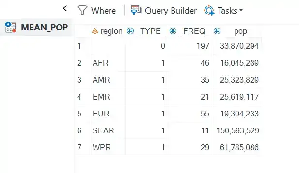
The OUTPUT statement creates a new dataset with the calculated statistics. For example, to create a dataset with the population for each region, the following code could be used:

PROC MEANS DATA = sashelp.demographics MEAN;
CLASS region;
VAR pop;
OUTPUT OUT = mean_pop mean=;
RUN;

Advanced Usage of PROC MEANS

Using PROC MEANS for Weighted Analysis

PROC MEANS can perform weighted analysis. For example, if a dataset contains a variable representing the number of similar houses in the area, this could be used as a weight in calculating the mean price:

data houses;
   input Area $ HousePrice NumHouses;
   datalines;
A 250000 10
B 300000 15
C 275000 8
D 320000 12
E 260000 9
;
run;
/* Use PROC MEANS for weighted analysis */
proc means data=houses mean sum;
   var HousePrice;
   weight NumHouses;
   title "Weighted Analysis of House Prices using Number of Houses as Weight";
run;

Using PROC MEANS for Percentile Analysis

PROC MEANS can also calculate percentiles. For example, to calculate the 25th, 50th, and 75th percentiles of house prices, the following code could be used:

PROC MEANS DATA = houses P25 P50 P75;
VAR HousePrice;
RUN;

Identifying Extreme Values

To get a correct analysis, excluding the observation containing the extreme lowest or extreme highest values is often necessary.

These extreme values are automatically displayed in PROC UNIVARIATE but must be explicitly specified in PROC MEANS and PROC SUMMARY procedures.

The MAX and MIN statistics show the extreme lowest or highest values, but it does not identify the observation which contains these extreme values.

MAXID and MINID

The two options- MAXID and MINID, when used in the OUTPUT statement, identify the observations with extreme values.

Example:

Let’s say we have a dataset named students that contains the scores of students in various subjects, and we want to identify the student with the highest and lowest score in mathematics.

Dataset students:

StudentID	Name	MathScore
1	John	85
2	Emily	92
3	Michael	78
4	Sarah	89

proc means data=students noprint;
	var MathScore;
	output out=stats max=maxScore min=minScore
	maxid(MathScore(name))=maxStudentName
	minid(MathScore(name))=minStudentName;
run;

proc print;

The above example shows that the output has been generated with extreme minimum and maximum values.

Using the IDGROUP Option to Identifying Extreme Values of Analysis Variables

THE IDGROUP option displays a group of extreme values, unlike the MAXID and MINID, which only captures a single extreme value.

The IDGROUP option in PROC MEANS is used to identify extreme values of analysis variables. It can be used to find the minimum, maximum, or both for the specified variables and to display the corresponding values of ID variables for those extreme values.

We can use the IDGROUP option in PROC MEANS to identify the top 2 students with the highest and lowest math scores:

data students;
   input StudentID Name $ MathScore;
   datalines;
1 John 85
2 Emily 92
3 Michael 78
4 Sarah 89
5 David 95
6 Olivia 88
7 Daniel 76
8 Sophia 93
9 William 82
10 Ava 90
;
run;

proc means data=students noprint;
   var MathScore;
   output out=ExtremeScores (drop= _freq_ _type_)
          idgroup(max(MathScore) out[2] (MathScore StudentID Name)=MaxScore) 
          idgroup(min(MathScore) out[2] (MathScore StudentID Name)=MinScore) 
          / autoname;
run;

proc print noobs;

After running the above code, the ExtremeScores dataset will contain the IDs and names of the students with the highest and lowest math scores.

The PERCENTILE to create subsets.

The percentile statistics are used to create search bounds for potential outlier boundaries. This can help us determine if any observation falls outside the defined percentile, like 1% or 5%.

The percentile is the data percentage below a certain point in the observation.

To compute the 25th, 50th (median), and 75th percentiles for the Score variable, you can use the following code:

data studentscores;
input StudentID $ Name $ Score;
datalines;
1 John 85
2 Emily 92
3 Michael 78
4 Sarah 89
5 David 91
6 Anna 84
7 Brian 88
8 Lisa 95
9 Tom 76
10 Jane 90
;
run;

proc means data=studentscores noprint;
	var Score;
	output out=percentile_results p25(Score)=Score_25th p50(Score)=Score_Median p75(Score)=Score_75th;
run;

proc print;

The output dataset percentile_results will contain the 25th, 50th, and 75th percentiles for the Score variable. These values are named Score_25th, Score_Median, and Score_75th respectively.

The p25, p50, and p75 options in the output statement of PROC MEANS are used to specify the desired percentiles. The (Score) after-each percentile option indicates the variable for which the percentiles are being calculated.

The automatic _TYPE_ variable

In PROC MEANS, the automatic _TYPE_ variable is created in the output dataset when you use the CLASS statement. The _TYPE_ variable provides information about the level of classification for each observation in the output dataset.

1. Value of 0: This indicates an overall summary statistic for the entire dataset, without any classification.
2. Values from 1 to n: If you have n class variables, _TYPE_ values from 1 to n represent individual class variables. The order corresponds to the order of the class variables in the CLASS statement.
3. Higher Values: Combinations of class variables are represented by higher values of _TYPE_. The value is determined by the combination of class variables used for that particular summary statistic.
4. Maximum Value: The maximum value of _TYPE_ (which is equal to the number of class variables) represents the summary statistic for the combination of all class variables.

data sampledata;
input Group $ Subgroup $ Value;
datalines;
A X 10
A Y 20
B X 30
B Y 40
;
run;

proc means data=sampledata noprint;
	class Group Subgroup;
	var Value;
	output out=means_output mean=ValueMean;
run;
proc print;

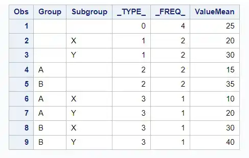
In the means_output dataset, the _TYPE_ variable will have the following values:

• _TYPE_ = 0: Represents the overall mean of the Value variable for the entire dataset.
• _TYPE_ = 1: Represents the mean of the Value variable for each Group.
• _TYPE_ = 2: Represents the mean of the Value variable for each Subgroup.
• _TYPE_ = 3: Represents the mean of the Value variable for each combination of Group and Subgroup.

Using the NWAY option

The NWAY option in PROC MEANS is used to produce summary statistics only for the highest level of interaction among the class variables. In other words, if you have multiple class variables, the NWAY option will only produce summary statistics for the combination of all class variables, and not for individual class variables or lower-level interactions.

Let’s consider a dataset with two class variables: Group and Subgroup.

data sampledata;
input Group $ Subgroup $ Value;
datalines;
A X 10
A Y 20
B X 30
B Y 40
;
run;

Now, let’s use PROC MEANS without the NWAY option:

title "Proc Means without Nway Option";
proc means data=sampledata noprint;
	class Group Subgroup;
	var Value;
	output out=means_output mean=ValueMean;
run;
proc print;

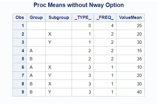
The output contains summary statistics for:

1. Overall data
2. Each Group
3. Each Subgroup
4. Each combination of Group and Subgroup

Now, let’s use PROC MEANS with the NWAY option:

title "Proc Means with the Nway Option";
proc means data=sampledata nway;
	class Group Subgroup;
	var Value;
	output out=nway_output mean=ValueMean;
run;
proc print;

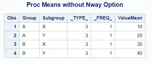
When using NWAY with CLASS variables in PROC MEANS, the output will only show the combination of all class variables, and not the individual levels or lower-level interactions.

Ways option

The WAYS option in PROC MEANS specifies the number of levels of interactions to display in the output. It’s used in conjunction with classification variables specified in the CLASS statement.

Let’s go through an example to understand the WAYS option:

Suppose we have a dataset of sales data for different products across various regions:

data sales;
input Product $ Region $ Sales;
datalines;
A North 100
A South 150
A East 110
A West 120
B North 90
B South 140
B East 105
B West 115
C North 80
C South 130
C East 100
C West 110
;

Now, let’s use PROC MEANS to compute the sum of sales for each combination of Product and Region:

Without the WAYS option:

proc means data=sales sum noprint;
   class Product Region;
   var Sales;
   output out=AllWays sum=;
run;

proc print data=AllWays noobs; run;

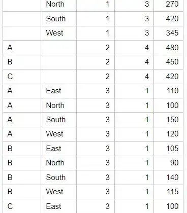
This will produce an output for all combinations: individual products, individual regions, and the combination of product and region.

Using the WAYS option:

proc means data=sales sum noprint;
   class Product Region;
   var Sales;
   ways 1;
   output out=OneWay sum=;
run;

proc print data=OneWay noobs; run;

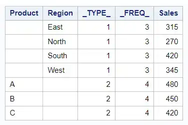
With WAYS 1, the output will only show the sum of sales for individual levels of the classification variables (i.e., individual products and individual regions) but not their combination.

If you use WAYS 2:

proc means data=sales sum noprint;
   class Product Region;
   var Sales;
   ways 2;
   output out=OneWay sum=;
run;

proc print data=OneWay noobs; run;

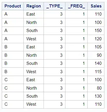
The output will show the sum of sales for two-way interactions (i.e., combinations of product and region).

In summary, the WAYS option allows you to control the levels of interactions displayed in the output when you have multiple classification variables.