Confidence Interval for Population Mean

In statistics, a confidence interval is a range of values that is likely to include the population parameter, and it is an essential tool for estimating population parameters based on sample data.

In this post, we will discuss the basics of confidence intervals, including their construction, interpretation, and application, with a focus on confidence intervals for population means. We will also provide examples and practical guidance on how to calculate and interpret confidence intervals using the standard deviation and sample mean.

A confidence interval constructed from sample data is a range of values that is likely to include the population parameter with a certain probability.

The objective of a confidence interval is to provide the location and precision of population parameters.

The confidence interval for the population mean may be stated as , which means the population mean lies between values of 30 and 50.

Since the true parameter estimate might or might not be in the interval estimate, we link confidence (probability) to finding the true parameter estimate in the interval.

We may say that there is a 95% confidence level that the interval contains the population mean, implying a 5% chance that the interval may not contain the population mean.

Confidence levels are usually written as 100% on the interval estimate of a population parameter, and it is the probability that the interval estimate will contain the true population parameter.

When ,95% is the confidence level, and 0.95 is the probability that the interval estimate will have the population parameter.

The value of is called significance which signifies the chance of not observing the true population means in the interval estimate.

Confidence Interval for Population Mean when Standard Deviation is known.

The confidence interval for a population mean is determined by taking the sample mean(point estimate) and adding or subtracting a margin of error from it.

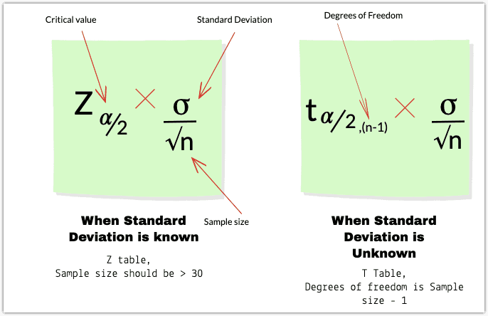
If the population Standard deviation is known, the margin of error is determined by

where and correspondingly,

So, if the CL = 95%

is called the critical value, which can be found in the Z table.

z value tells us how many Standard deviations an observation is from the mean. A Z score of -2 tells us that the observation is 2 Standard deviations to the left of the mean.

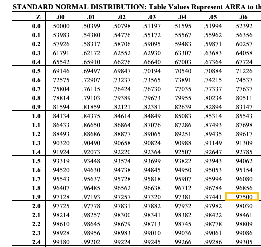
More specifically, it allows us to calculate how much area a specific Z score is associated with. We can find the exact area using a Z table, also known as the Standard Normal Table.

The table shows the total area on the left side of any value of Z.

The Top row and the first column correspond to the Z value and all the numbers in the middle correspond to the areas.

Let’s find the Z value for a 95% confidence interval.

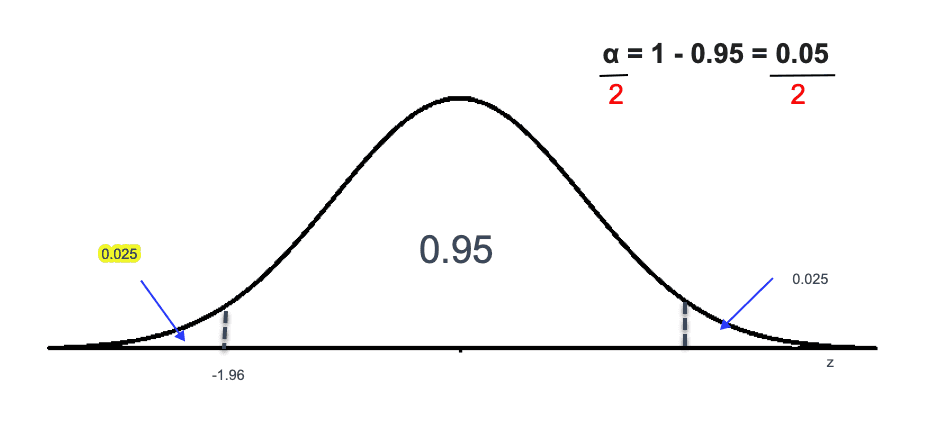
We know that = 0.05 for a 95% confidence interval. The total area represents 1. Since 95% or 0.95 is the area in the middle and the leftover area is the , we have to divide into two equal parts, which will correspond to 0.025 area to the left and 0.025 area to the right.

So, the area to the left will be 0.95 + 0.025 = 0.975. We can calculate the Positive Z value by looking at the Z table and finding the area closest to 0.975, which is 1.96.

This Z value tells us that 95% of the area lies with roughly 1.96 standard deviations from the mean.

Since the normal distribution is symmetrical, the corresponding value to the left of the curve will be -1.96.

We can write the 95% confidence interval for the population mean when the population standard deviation is known as :

Example:

A sample of 100 subjects was chosen to estimate the length of stay at a hospital. The sample mean was 4.5 days and the population standard deviation was 1.2 days.

1. Calculate the 95% confidence interval for the population means.
2. What is the probability that the population means is greater than 4.73 days?

Solution:

(1) Known Values are:

days =1.2

The estimated value of mean from a sample size can be calculated using

and we know that Margin of Error and thus the formula can be written as:

So,

The 95% confidence interval is given by:

where 1.96 is the critical value obtained from the Z table for a 95% confidence Interval where = 0.0975 and 0.025

Thus, to interpret this, we can say that we are 95% confident that the population means is between 4.2648 and 4.7352.

(2) Since the upper limit of 95% confidence interval is 4.7352, we can say that the probability of a population means greater than 4.7352 is approximately 0.025.

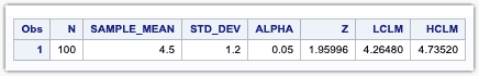
Calculating the Confidence Interval in a SAS data step

The confidence interval can be calculated in a SAS data step as below.

data CI;
 N=100;
 SAMPLE_MEAN=4.5;
 STD_DEV=1.2;
 ALPHA=0.05;
 Z =probit(1-ALPHA/2);
 LCLM=SAMPLE_MEAN-Z*STD_DEV/SQRT(N);
 HCLM=SAMPLE_MEAN+Z*STD_DEV/SQRT(N);
run;

Refer to the article to learn how you can use SAS procedures to calculate confidence intervals in SAS.

Confidence Interval for Population Mean when Standard Deviation is unknown.

When the confidence interval is unknown, we will not be able to use the below formula.

William Gossett proves that if the population follows a normal distribution and the standard deviation is calculated from the sample, the statistics below will follow a t-distribution with (n-1) degrees of freedom.

S is the standard deviation estimated from the sample. The t-distribution is almost similar to the standard normal distribution. It has a bell shape, and its mean median and mode equal 0.

The major difference between t-distribution and standard normal distribution is that t-distribution has a broad tail compared to standard normal distribution. However, as the degrees of freedom increase, the t-distribution converges to a standard normal distribution.

The confidence interval mean from a population that follows a normal distribution when the standard deviation is unknown is given by

Example :

An online grocery store is interested in estimating the basket size of its customer orders to optimize the size of crates used for delivering the grocery items. For a sample size of 70 customers, the basket size was 24, and the standard deviation estimated from its sample was 3.8. Calculate the 95% confidence interval for the basket size of the customer order.

Solution:

degrees of freedom is (n-1) = 69

The T-value can be found using the T table or the TINV function in SAS.

Using the T-table, you have to look at the intersection of degrees of freedom for the corresponding Confidence Level.

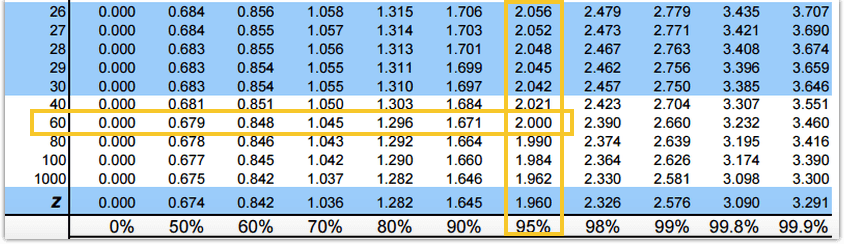
Since the degrees of freedom 69 is not available, we have to look for the closest value of 69, which is 60, and the corresponding T value is 2.000.

The confidence, interval for the size of the basket is given by

The Lower confident limit is given by

The Upper confident limit is given by

Thus, the 95% confidence interval for the size of the basket is (23.09,24.91)

Calculating Confidence Interval in SAS

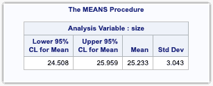
We can use the PROC MEANS procedure with the CLM option in SAS to find the Lower and Upper Confidence limits.

I have simulated the above example using random numbers and calculated below the Lower and Upper Confidence limits.

data basket;
 do i=1 to 70;
  size=round(20+ floor(1+30-20)*rand("uniform"), .01);
  output;
 end;
 drop i;
run;
proc means alpha=0.05 clm mean std maxdec=3; 
var size; 
run;

If you don’t have the raw data, you can also use the below data step to calculate the Confidence Limit.

data CI;
 X=24;
 S=3.8;
 N=70;
 ALPHA=0.05;
 CRITICAL_VALUE=TINV(1-ALPHA/2, N-1);
 LCLM=X - (CRITICAL_VALUE * S/sqrt(N) );
 HCLM=X + (CRITICAL_VALUE * S/sqrt(N) );
run;

Conclusion

Confidence intervals are essential in statistics for estimating population parameters from sample data. In this post, we have covered the basics of confidence intervals for population means, including their construction, interpretation, and practical application. By using confidence intervals, you can ensure that your research is more accurate, reliable, and actionable.