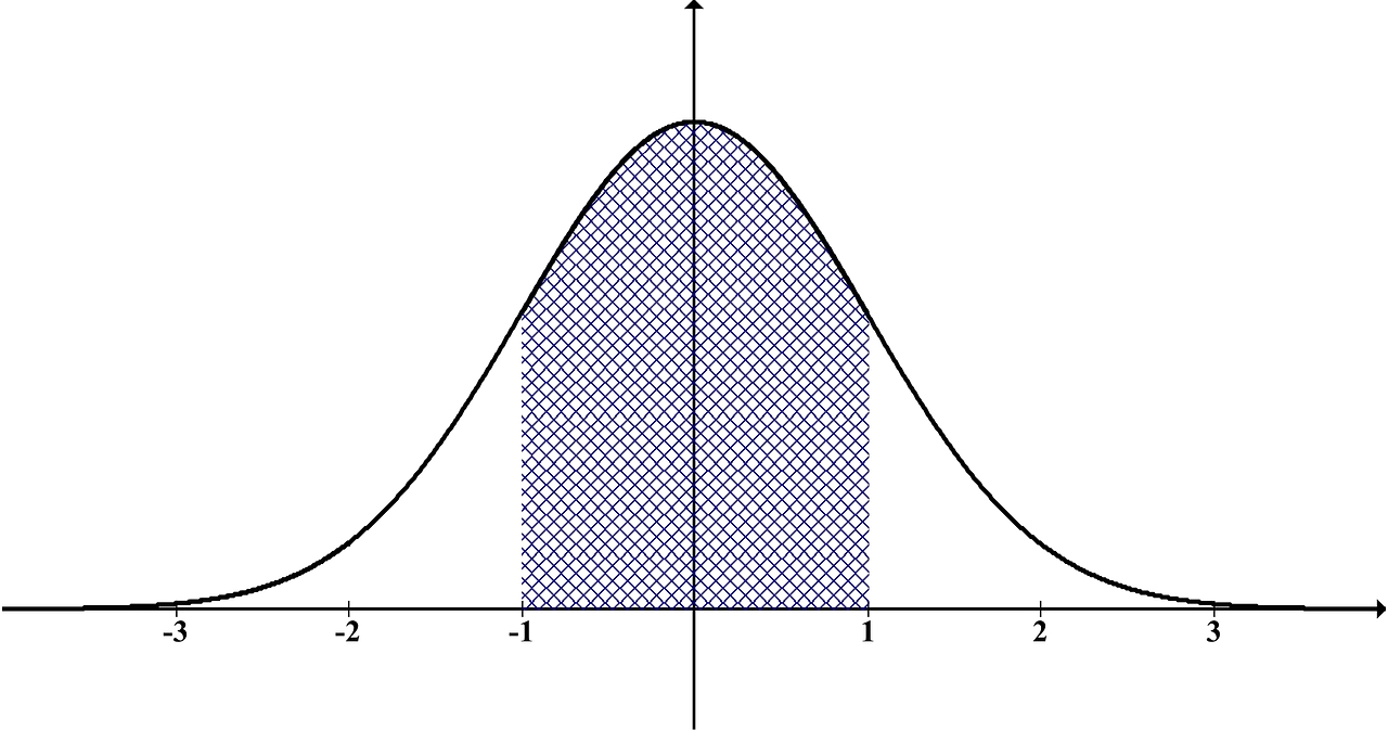
Descriptive Statistics In SAS With Examples

Descriptive Statistics is about finding “what has happened” by summarizing the data using statistical methods and analyzing the past data using queries.

Descriptive statistics, in short, are descriptive information that summarizes a given data. The input data can be either a representation of the entire population or a subset of a population.

Descriptive statistics are of two types, measures of central tendency and variability.

The tools and techniques used for describing or summarizing the data in descriptive statistics are:

Measures of Central Tendency	MEAN, MEDIAN and MODE
Measures of Variance	Range, Inter-Quartile Distance, Variance, Standard Deviation
Measures of Shape	Skewness and Kurtosis

Measures of Central Tendency

In Descriptive Statistics, measures of central tendency are used to describe the data using a single value. It helps users to summarize the data.

Mean

Mean is one of the measures of central tendency used in descriptive statistics. It is the arithmetic average value of the data, calculated by adding all data observations and dividing by the number of observations.

Example :

Age

The average age (MEAN) of students from the above sample is given by

$\overline{X}=\frac{21+22+23+24}{4}=22.5$

Limitations

The mean is significantly affected by the presence of outliers. Therefore, it is not a useful measure in taking decisions.

$\overline{X}=\frac{21+22+23+200}{4}=66.5$

Median

The Median in descriptive statistics is the value that divides the data into two equal parts. To find the median value, the data must be arranged in ascending order, and the median is the value at position $(n+1/2 )$ when $n$ is odd.

When $n$ is even, the median is the average value of $(n/2)^2{th}$ and $(n+2)/2^{th}$ observation after arranging the data in an increasing order.

Example:

245

326

180

226

445

319

260

The ascending order of the data is 180,226,245,260,319,326,445.

Now, $\frac{(n+1)}{2}=\frac{8}{2}=4$

Thus, the median is the 4^th value in the data, 260, after arranging in ascending order.

Calculating Mean and Median in SAS

PROC MEANS can find the mean and median in a SAS dataset.

title 'Table of Mean and Median for Students age';
proc means data=sashelp.class mean median maxdec=2; 
var age;
run;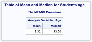

MODE

A mode is a value that occurs more frequently in the data set.

Calculating Mode in SAS

The mode of a dataset can be calculated in SAS using the PROC UNIVARIATE procedure.

title 'Table of Modes for Student age';
ods select Modes;
proc univariate data=sashelp.class modes; 
var age;
run;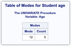

PERCENTILE, DECILE, AND QUARTILE

Percentile, decile, and Quartile are frequently used to identify the observation position in a SAS dataset.

The percentile is used to identify the position of any value in a group. The percentile is denoted as P $x$ , which is the value of the data at which $x$ percentage of the data lies below that value.

P₁₀ denotes the value below which 10 percent of the data lies. To find P $x$ , arrange the data in ascending order, and the value of P $x$ is the position in the data is calculated using the below formula.

P $x$ $\approx \frac{x(n+1)}{100}$

$n$ is the number of observations in the data.

Calculating percentile in SAS

The frequently used percentiles (such as the 5th, 25th, 50th, 75th, and 95th percentiles) can be calculated using PROC MEANS. The STACKODSOUTPUT option was introduced in SAS 9.3 to create an output data set containing multiple variables’ percentiles.

proc means data=sashelp.cars StackODSOutput P5 P25 P75 P95; 
var mpg_city mpg_highway; 
ods output summary=Percentiles;
run;

Descriptive Statistics in SAS with Examples

DECILE

The decile is the percentile value that divides the data into ten equal parts. The first decile contains 10% of the data, the second decile contains the first 20% of the data and so on.

QUARTILE

Quartile divides the data into four equal parts. The first Quartile (Q1) contains 25% of the data, Q2 contains 50% of the data and the median. Q₃ contains 75% of the data.

Measures of Variation

In Descriptive statistics, Measures of Variations help us understand the data’s variability. Predictive analytics, like Regression, explains variations in the outcome variable(Y) using the predictor variable (X). variability in the data is measured using the following techniques.

Range
Inter Quartile Distance (IQD)
Variance
Standard Deviation

RANGE

RANGE captures the data spread and is the difference between the maximum and minimum value of the data.

Calculating RANGE in SAS

Proc means can be used with the RANGE option to calculate the RANGE of any variables.

proc means data=sashelp.class range maxdec=2; 
var age weight;
run;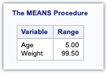

INTER-QUARTILE DISTANCE (IQD)

Inter-Quartile Distance, also known as Inter-Quartile Range (IQR), is the measure of the distance between Quartile 1 (Q₁) and Quartile 3 (Q₃).

IQD can also be used for identifying outliers in the data. Outliers are observations that are far away (on either side) from the mean value of the data.

Data values below Q₁ – 1.4 * IQD and above Q₃ + 1.5 * IQD are classified as outliers.

SAS program to find Outliers using the IQD

data class; 
set sashelp.class; 
if name in('Alice', 'Carol', 'Henry') then age=110 + rand("Uniform");
run;

proc univariate data=class noprint; 
var age; output out=ClassStats qrange=iqr q1=q1 q3=q3;
run;

data _null_; 
set classStats; 
call symput ('iqr', iqr); 
call symput ('q1', q1); 
call symput ('q3', q3);
run;

data outliers; 
set class; 
if (age le &q1 - 1.5 * &iqr) or (age ge &q3 + 1.5 * &iqr);
run;

proc print data=outliers;
run;

In the above program, we have modified it as help.class dataset by inserting some outlier age.

Then, QRANGE, Q1 and Q3 are calculated for the modified SAS dataset.

Macro variables are created for the three variables, respectively.

Conditions are applied to the modified dataset ‘class’ to check for outliers.

VARIANCE

Variance is a measure of variability in the data from the mean value.

The variance of a population $\sigma^2$ ,is calculated using

$\sigma^2=\sum_{i=1}^n frac{(X_i - mu^2)}{n}$

The variance of a sample is ( $S^2$ ) is calculated using

$S^2=\sum_{i=1}^n \frac{(X_i - \overline{X}^2)}{n-1}$

Note that the deviation from the mean is squared since the sum of deviations from the mean will always add up to 0.

For calculating sample variance, the sum of squared deviation is divided by $n-1$ . This is known as Bessel’s correction.

STANDARD DEVIATION

Standard deviation is the square root of Variance and is also a measure of how spread out the numbers are from the mean value.

Why do we need a Standard Deviation?

Since variance is the square of deviations, it does not have the same unit of measurement as the original values.

For example, lengths measured in metres ( $m$ ) have a variance measured in metres squared ( $m^2$ ).

Finding the square root of the variance gives us the units used in the original scale, which is known as the standard deviation.

The formula of Standard deviation for the population is

$\sigma=\sum_{i=1}^n \frac{(X_i - mu^2)}{n}$

and for Sample is

$S=\sum_{i=1}^n \frac{(X_i - \overline{X}^2)}{n-1}$

Properties of standard deviation

Standard deviation is used to measure the spread of data around the mean.
Standard deviation can never be negative as it is a measure of distance (and distances can never be negative numbers).
Standard deviation is significantly affected by outliers.
For data with approximately the same mean, the greater the spread is, the greater the standard deviation.
The standard deviation is zero (the smallest possible number in Standard deviation) if all dataset values are the same(This is because each value is equal to the mean).

Calculating Variance and Standard Deviation in SAS

Variance and Standard deviation can be calculated using the VAR and STDDEV options in the PROC MEANS Procedure.

proc means data=sashelp.class; 
var stddev maxdec=2; 
var age;
run;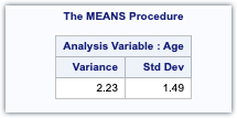

MEASURES OF SHAPE – SKEWNESS AND KURTOSIS

SKEWNESS is a measure of symmetry or lack of symmetry. A data set is symmetrical when the proportion of data at an equal distance from the mean is equal.

Measures of skewness are used to identify whether the distribution is left-skewed or right-skewed.

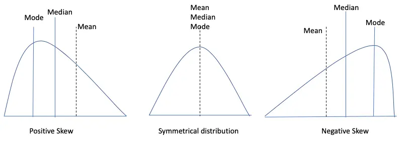
The value of Skewness will be 0 when the data is symmetrical. A positive value indicates a positive skewness, whereas a negative value indicates negative skewness.

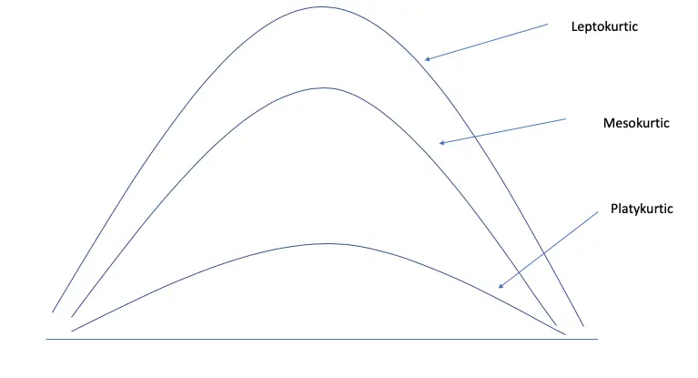
KURTOSIS is a measure of the shape of the tail, i.e. the shape of the tail of a distribution is heavy or light.

Kurtosis identifies whether the tails of a given distribution contain extreme values.

Excess Kurtosis

Excess kurtosis is a measure that compares the kurtosis of distribution by subtracting the kurtosis of a normal distribution. The kurtosis of a normal distribution is 3. Therefore, the excess kurtosis is found using the formula below:

Excess Kurtosis = Kurtosis – 3

Types of Kurtosis

The types of kurtosis are determined by the excess kurtosis of a particular distribution. The excess kurtosis can be positive, negative or 0.

Leptokurtic Distribution

A kurtosis value of more than three is called Leptokurtic distribution. The leptokurtic distribution has heavy tails on either side, indicating large outliers.

Platykurtic Distribution

A kurtosis value of less than three is called Platykurtic distribution. It shows a negative excess kurtosis which has flat tails. The flat tails indicate the presence of small outliers in a distribution.

Mesokurtic Distribution

The Kurtosis value equal to 3 is called Mesokurtic distribution, which shows an excess kurtosis of 0 or close to 0.

Calculating Kurtosis and Skewness in SAS

Skewness and Kurtosis are calculated using the PROC UNIVARIATE procedure in SAS.

proc univariate data=sashelp.class; 
var age;
run;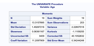

In the above example, the Skewness is close to 0, meaning age values are almost normally distributed. The Kurtosis value is negative, meaning that age values are flatter than a normal curve with the same mean and standard deviation.

If you liked this article, you might also want to read How to summarize categorical data graphically?

Do you have any tips to add? Let us know in the comments.

Please subscribe to our mailing list for weekly updates. You can also find us on Instagram and Facebook.

Descriptive Statistics in SAS with Examples

Measures of Central Tendency

Mean

Median

Calculating Mean and Median in SAS

MODE

Calculating Mode in SAS

PERCENTILE, DECILE, AND QUARTILE

Calculating percentile in SAS

DECILE

QUARTILE

Measures of Variation

RANGE

Calculating RANGE in SAS

INTER-QUARTILE DISTANCE (IQD)

SAS program to find Outliers using the IQD

VARIANCE

STANDARD DEVIATION

Why do we need a Standard Deviation?

Properties of standard deviation

Calculating Variance and Standard Deviation in SAS

MEASURES OF SHAPE – SKEWNESS AND KURTOSIS

Excess Kurtosis

Types of Kurtosis

Leptokurtic Distribution

Platykurtic Distribution

Mesokurtic Distribution

Calculating Kurtosis and Skewness in SAS

Subhro

Leave a ReplyCancel reply

Measures of Central Tendency

Mean

Median

Calculating Mean and Median in SAS

MODE

Calculating Mode in SAS

PERCENTILE, DECILE, AND QUARTILE

Calculating percentile in SAS

DECILE

QUARTILE

Measures of Variation

RANGE

Calculating RANGE in SAS

INTER-QUARTILE DISTANCE (IQD)

SAS program to find Outliers using the IQD

VARIANCE

STANDARD DEVIATION

Why do we need a Standard Deviation?

Properties of standard deviation

Calculating Variance and Standard Deviation in SAS

MEASURES OF SHAPE – SKEWNESS AND KURTOSIS

Excess Kurtosis

Types of Kurtosis

Leptokurtic Distribution

Platykurtic Distribution

Mesokurtic Distribution

Calculating Kurtosis and Skewness in SAS

Subhro

Leave a ReplyCancel reply

You Might Also Like

How to Copy a file with SAS?

Working with SAS libraries

How to choose a statistical test?